|
|
| Zeile 19: |
Zeile 19: |
| | ==Allgemeine lineare Gleichung mit zwei Variablen== | | ==Allgemeine lineare Gleichung mit zwei Variablen== |
| | *[[Allgemeine lineare Gleichung mit zwei Variablen]] | | *[[Allgemeine lineare Gleichung mit zwei Variablen]] |
| − | ===ax + by + c = 0===
| |
| − | <math>
| |
| − | \begin{align}
| |
| − | ax+by=c \\
| |
| − | a, b, c \in \mathbb{R} \\
| |
| − | x, y \in \mathbb{R},
| |
| − | \end{align}
| |
| − | </math><br />
| |
| − | <iframe scrolling="no" title="Lineare Gleichung mit zwei Variablen" src="https://www.geogebra.org/material/iframe/id/ScDQeGnF/width/852/height/568/border/888888/smb/false/stb/false/stbh/false/ai/false/asb/false/sri/false/rc/false/ld/false/sdz/false/ctl/false" width="852px" height="568px" style="border:0px;"> </iframe>
| |
| − | <br />
| |
| − | ===Grafische Veranschaulichung der Lösungsmenge einer Gleichung vom Typ ax+by=c===
| |
| − | Es seien <math>a, b, c \in \mathbb{R}</math> , beliebig aber fest, <math>a, b</math> nicht gleichzeitig <math>0</math>,<br />
| |
| − | <math>x,y \in \mathbb{R}</math>, variabel.<br /> Wir untersuchen die Gleichung<br />
| |
| − | (I) <math>ax+by=c</math>
| |
| | | | |
| − | '''Satz 1:'''<br />
| |
| − | :Die Gleichung (II) <math>ax+by=c</math> beschreibt die Menge aller Punkte einer Geraden in der reellen Zahlenebene.<br />
| |
| − | '''Beweis:'''<br />
| |
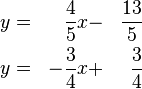
| − | Aus der Schule ist die folgende Gleichung für Geraden bekannt: <math>y=mx+b</math>, <math>m,b \in \mathbb{R}</math>, beliebig aber fest, <math>x,y \in \mathbb{R}</math> variabel.
| |
| − | Wir führen zwei Beweise:
| |
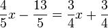
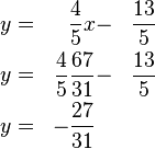
| − | # Wir zeigen, dass jede Gleichung vom Typ (I) durch äquivalente Umformungen in eine Gleichung vom Typ (II) überführt werden kann.
| |
| − | # Wir zeigen, dass umgekehrt (fast) jede Gleichung vom Typ (II) durch äquivalente Umformungen in den Typ (I) überführt werden können.
| |
| − | Ausführung des Beweises: Übungsaufgaben 1.1 und 1.2 in [[Serie 1: Geraden in der Ebene, zwei Gleichungen mit zwei Unbekannten SoSe 2018]]
| |
| − | ===Algebraische Beschreibung der Lösungsmenge einer Gleichung der Form <math>ax+by=c</math>===
| |
| − | ====Voraussetzung====
| |
| − | Wir schließen aus, dass <math>a</math> und <math>b</math> gleichzeitig <math>0</math> sind: <math>a^2 +b^2 \not = 0</math>
| |
| − | ====Fall 1: <math>b \not =0</math>====
| |
| − | <math>
| |
| − | \begin{align}
| |
| − | ax+by &= c \\
| |
| − | by &= -ax+c \\
| |
| − | y &= \frac{-ax+c}{b} \\
| |
| − | y &= -\frac{a}{b}x+\frac{b}{c}
| |
| − | \end{align}
| |
| − | </math>
| |
| − | <br />
| |
| − |
| |
| − | <math>L=\left \{ (x\vert y) \left \vert \begin{align} x&= t \\ y&= -\frac{a}{b}t+\frac{b}{c} \end{align} ; t \in \mathbb{R} \right. \right \}</math><br />
| |
| − | Falls <math>a=0</math> vereinfacht sich die Lösungsmenge <math>L</math> zu: <br />
| |
| − | <math>L=\left \{ (x\vert y) \left \vert \begin{align} x&= t \\ y&= \frac{b}{c} \end{align} ; t \in \mathbb{R} \right. \right \}</math><br />
| |
| − |
| |
| − | ====Fall 2: <math>b=0</math>====
| |
| − | <math>
| |
| − | \begin{align}
| |
| − | a x &=c \\
| |
| − | x&=\frac{c}{a}
| |
| − | \end{align}
| |
| − | </math><br />
| |
| − | <math>L=\left \{ (x\vert y) \left \vert \begin{align} x&= \frac{c}{a} \\ y&= t\end{align} ; t \in \mathbb{R} \right. \right \}</math><br />
| |
| − |
| |
| − | ==Zusammenfassung==
| |
| − | # <math>a \not = 0 \land b \not = 0</math> :Gerade, die weder zur <math>x-</math> noch zur <math>y-</math>Achse parallel ist.
| |
| − | # <math>a = 0 \land b \not = 0</math> : Gerade, die parallel zur <math>x-</math>Achse ist.
| |
| − | # <math>a \not = 0 \land b = 0</math> : Gerade, die parallel zur <math>y-</math>Achse ist.
| |
| | | | |
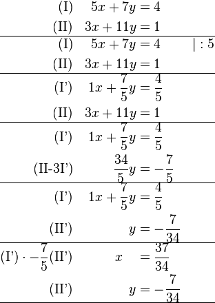
| | ==Lösen eines linearen Gleichungssystems mit zwei Gleichungen und zwei Unbekannten== | | ==Lösen eines linearen Gleichungssystems mit zwei Gleichungen und zwei Unbekannten== |
 um:
um: