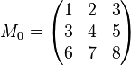
Die Koeffizientenmatrix
So ist es, wenn man sich schnell in der Vorlesung ein Gleichungssystem einfallen lässt.
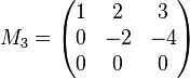
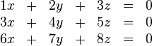
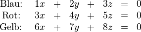
Zur Erinnerung: an der Tafel entstand spontan eine Koeffizientenmatrix vom folgenden Typ:
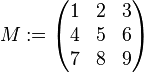 Wir wollten den Rang (die Anzahl der linear unabhängigen Zeilen) dieser Matrix bestimmen und waren zunächst davon überzeugt, dass diese spezielle Wahl darauf hinaus laufen müsste, dass alle die Zeilen der Matrix
  linear unabhängig sein würden und unsere Matrix damit den Rang linear unabhängig sein würden und unsere Matrix damit den Rang  haben würde.
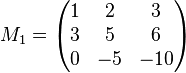
Völlig erstaunt waren wir als wir konstatieren mussten, dass die dritte Zeile eine Linearkombination der ersten beiden Zeilen ist. Natürlich kann man den Algorithmus zur Generierung der Diagonalenform der Matrix anwenden, so wie wir es taten. Mehr Überzeugungskraft hat jedoch die Betrachtung des Schemas, wie die Matrix entsteht: haben würde.
Völlig erstaunt waren wir als wir konstatieren mussten, dass die dritte Zeile eine Linearkombination der ersten beiden Zeilen ist. Natürlich kann man den Algorithmus zur Generierung der Diagonalenform der Matrix anwenden, so wie wir es taten. Mehr Überzeugungskraft hat jedoch die Betrachtung des Schemas, wie die Matrix entsteht:
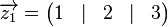


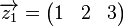
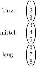
Den Zeilenvektor 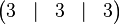 bezeichnen wir kurz mit bezeichnen wir kurz mit  . .
Damit können wir wie folgt schreiben: 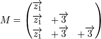 . .
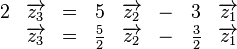
Jetzt sieht man leicht, dass  eine Linearkombination von eine Linearkombination von  und und  ist: ist:
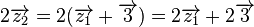
 . .
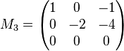
war die Matrix, die ich eigentlich an die Tafel bringen wollte. Stattdessen schrieb ich 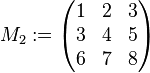 . Der Beweis für . Der Beweis für  funktioniert analog. Überzeugen Sie sich davon. Viel Spaß dabei --*m.g.* (Diskussion) 15:55, 24. Mai 2018 (CEST) funktioniert analog. Überzeugen Sie sich davon. Viel Spaß dabei --*m.g.* (Diskussion) 15:55, 24. Mai 2018 (CEST)
Die Matrix aus der Vorlesung
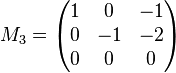
Die 3.Zeile ist eine Linearkombination der beiden anderen Zeilen


Also:
ist damit eine Linearkombination der Vektoren und .
Die beiden oberen Zeilen sind linear unabhängig
Bei der Untersuchung der linearen Unabhängigkeit von zwei Zeilen geht es nur darum, ob eine Zeile aus der anderen Zeile durch Multiplikation mit einer reellen Zahl hervorgeht:
Gesucht ist also  mit mit 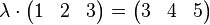
Eine solche Zahl  existiert nicht. Zeile 1 und Zeile 2 bilden zusammen eine Menge linear unabhängiger Zeilenvektoren. existiert nicht. Zeile 1 und Zeile 2 bilden zusammen eine Menge linear unabhängiger Zeilenvektoren.
Der Rang der kleinen Koeefizientenmatrix
Die Matrix hat damit den Rang  : :
Die Anzahl der linear unabhängigen Zeilenvektoren der Menge  ist 2. ist 2.
Die mehr algorithmische Vorgehensweise aus der Vorlesung
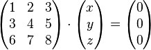
Ausgangsmatrix
Schritt 1
Zeile 1 mit  multiplizieren und dann zu Zeile 3 addieren. multiplizieren und dann zu Zeile 3 addieren.


Wir erhalten die folgende Matrix:
Schritt 2
Zeile 1 mit  multiplizieren und zu Zeile 2 addieren: multiplizieren und zu Zeile 2 addieren:


Wir erhalten die folgende Matrix:
Schritt 3
Wir multiplizieren die zweite Zeile aus mit  und addieren sie dann zu Zeile 3 in und addieren sie dann zu Zeile 3 in


Wir erhalten die folgende Matrix:
Der Rang unserer Ausgangsmatrix (wie der Matrix  ) kann damit nicht mehr sondern nur noch höchstens sein. ) kann damit nicht mehr sondern nur noch höchstens sein.
Schritt 4
Wir addieren die zweite Zeile der Matrix zur ersten Zeile der Matrix und erhalten:
Wir vereinfachen:
Weitere Vereinfachungen sind nicht mehr möglich, unsere Matrix hat den Rang 2.
Geometrische Interpretation der Matrix und des LGS
Lösungsgerade
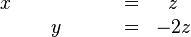
Wir ergänzen zum sogenannten homogenen LGS:
bzw.
Da wir das homogene LGS betrachten, können wir auch unmittelbar die vereinfachten Matrizen verwenden:
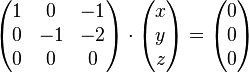
bzw.
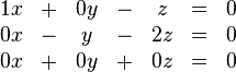
oder noch einfacher:
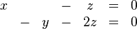
bzw.
Es ergibt sich damit die folgende Lösungsmenge  für unser homogenes LGS: für unser homogenes LGS:
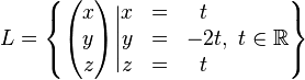
Wir erkennen einen proportionalen Zusammenhang jeweils zwischen den  Werten, Werten,  Werten und Werten und  Werten. Werten.
Die Lösungsmenge lässt sich also als die Menge der Koordinaten der Punkte einer Geraden  interpretieren. Diese Gerade geht u.a. durch die Punkte interpretieren. Diese Gerade geht u.a. durch die Punkte  und und  . Wir schreiben die Gleichung der Geraden in Parameterform: . Wir schreiben die Gleichung der Geraden in Parameterform:  mit mit  und und 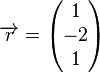 und damit und damit 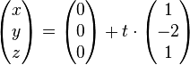
Grafische Darstellung der Lösungsgeraden in Geogebra
nur die Gerade
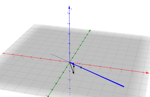
Lösungsgerade auf Geoegebra Tube
mit den Ebenen der vereinfachten Koeffizientenmatrix
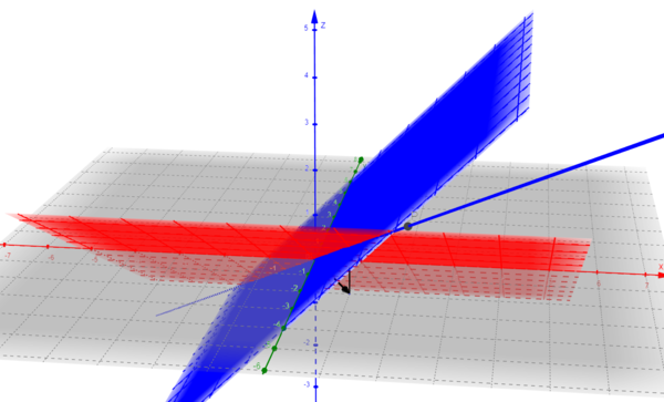
Lösungsgerade mit einfachen Ebenen auf Geoegebra Tube
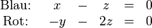
mit den Ebenen der Ausgangsmatrix und den Normalenvektoren der Ausgangsebenen
Ebenen
Normalenvektoren
Die Datei auf Geogebra Tube
Wir sehen, dass die drei Normalenvektoren komplanar sind. Sie können Sich die Ebene in der Geogebradatei anzeigen lassen (Ebene f).
| 

